Recommender Systems – Collaborative Filtering From Scratch

NOTE: All symbols used and their meaning, even though provided then and there are also provided in a chart at the end. Also the Kaggle notebook can be found here –
https://www.kaggle.com/code/innomight/recommender-system-collaborative-filtering/notebook

Lets Start!

This one will tell you how recommender systems work and how you can create one yourself.
This will also help you understand Collaborative Filtering vs Content Based filtering in recommender systems and how content based filtering solves some problems that we face while using collaborative filtering. To know and understand how you get movie / video / book recommendations in apps like netflix, youtube, amazon etc. keep reading.

Collaborative filtering = “People like you liked this”
Content-based = “You liked similar things before”

NOTE: Everything discussed in this blog and every material used can be found in the kaggle notebook attached. (Refer to the notebook to understand notations and functions)

Now, we will be building it from scratch so pay attention –

Let us start with collaborative filtering – It does not care about movie genres or types etc. It only cares about “Users who behaved similarly in the past will behave similarly in the future”

User A liked Movie X
User B liked Movie X

It concludes:

Users A and B are similar
So recommend A what B likes

Collaborative Filtering –

Cost Function –

We can think of collaborative filtering as solving two optimization problems simultaneously:

Learning user preferences while keeping movie features fixed
Learning movie features while keeping user preferences fixed

Each of these has its own cost function, but both share the same prediction term.

When combined, they form a single unified objective function that jointly learns both user and movie representations. This unified formulation is what we optimize using gradient descent in practice.

Equation 1: Learn User Preferences

$J(\theta^{(j)}) = \frac{1}{2} \sum_{i: r(i,j)=1} \left( (\theta^{(j)})^T x^{(i)} – y^{(i,j)} \right)^2 + \frac{\lambda}{2} \sum_k (\theta_k^{(j)})^2$

Equation 2: Learn Movie Features

$J(x^{(i)}) = \frac{1}{2} \sum_{j: r(i,j)=1} \left( (\theta^{(j)})^T x^{(i)} – y^{(i,j)} \right)^2 + \frac{\lambda}{2} \sum_k (x_k^{(i)})^2$

Combined Objective

$J(X, \Theta) = \frac{1}{2} \sum_{(i,j): r(i,j)=1} \left( (\theta^{(j)})^T x^{(i)} – y^{(i,j)} \right)^2 + \frac{\lambda}{2} \left( \sum_i ||x^{(i)}||^2 + \sum_j ||\theta^{(j)}||^2 \right)$

We are now implementing: $J = \frac{1}{2} \sum_{i,j: r(i,j)=1} \left( (\theta^{(j)})^T x^{(i)} – y^{(i,j)} \right)^2$

What we are actually doing is –
Predict rating
Compare with actual rating
Square the error Sum over all known ratings

For every movie i and for every user j

If rating exists:
error=prediction−actual

Lets make this clearer –
Think of it like this –

X = Movie Features
For Example:

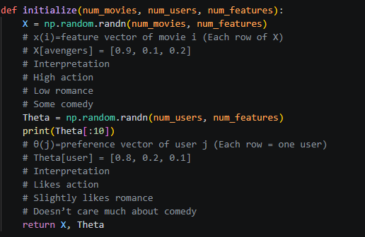
As you can see in above screenshot – X[avengers] this means the features belonging to this particular move and Theta is user preference Theta[user].
If a user likes Avengers for example the resultant dot product would be higher in value as 0.8 * 0.9 + …. all the features multiplied with user preference toward that feature gives us a scaler determining how much this user likes this movie.

Collaborative filtering can be viewed as a matrix factorization problem, where the ratings matrix is decomposed into two lower-dimensional matrices: one representing item features and the other representing user preferences. The dot product between these representations reconstructs the observed ratings.

Now moving on to compute cost function – Read comments to understand smaller things as well.

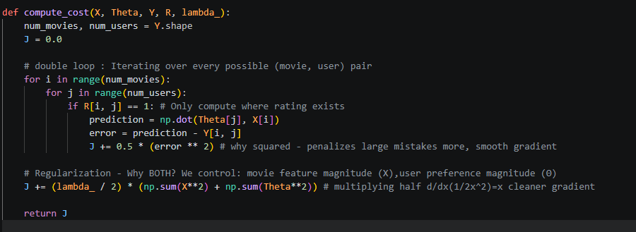
What we are doing –
For every movie i, user j:
– Add to total cost
– Predict rating
– Compare with actual
– Square the error

Right now Theta and X are random so Cost J returned is random and high.

Note from this section – The cost function measures the discrepancy between predicted and actual ratings, but only over observed entries. A regularization term is added to prevent the model from assigning excessively large values to the latent features, ensuring better generalization.

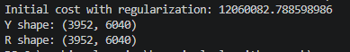
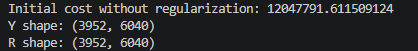
Just for insights here are cost functions at initial stage with random values with and without regularization

Right now:

Error term dominates (very large)
Regularization is relatively small

Later during training:

Regularization becomes very important

Also, do not get shocked by such big of a cost – 12 million because it we initialize –
X = 0.01 * random
Theta = 0.01 * random
Prediction:
θ⋅x ≈ verysmall(0)
Actual ratings: 1–5

So error ≈ 2–4

Squared error ≈ 4–16

Multiply by 1M entries → large cost (We are using Movielens dataset therefore 1 million entries)
We will calculate RMSE (Root Mean Squared Error Later) because I just didnt want to.

Let us move on to a very important topic – Gradients

Gradients

The gradients reveal how each user-item interaction influences both the item representation and the user preference vector. Each observed rating contributes to updating both entities, making collaborative filtering a jointly learned system.

Collaborative Filtering – Matrix Factorization version of linear regression

Collaborative filtering can be interpreted as performing a separate linear regression for each user, where the movie features act as inputs and user preference vectors act as weights. However, unlike traditional regression, both the inputs and the weights are learned simultaneously.

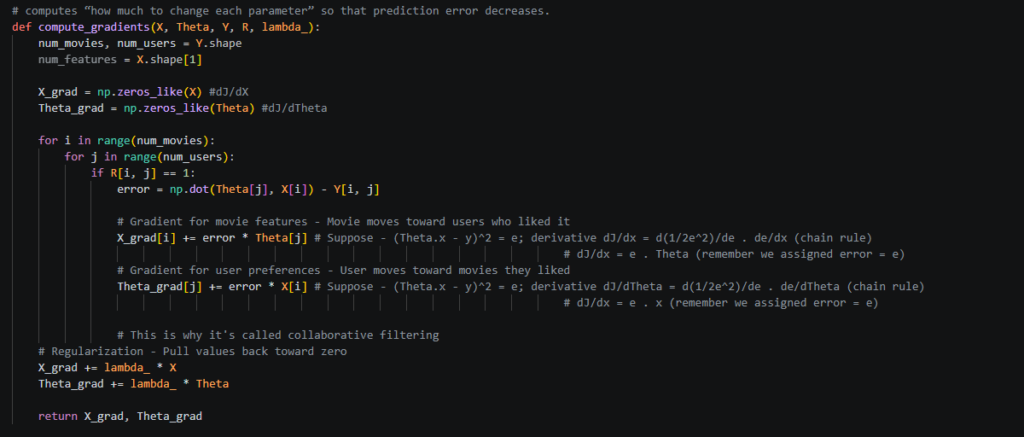
In the above screenshot, you can see how we compute gradients. Read the comments carefully as they explain how we land at the resultant error * theta[j] for X gradient and error * X[i] for Theta gradient.

Now, lets use simple words what is gradient and why are we calculating it.

We calculated cost (very high initially), we want to reduce the cost, right because cost J tells how wrong the model is. So, J = how wrong the model is. Now, Gradients (Delta J) X_grad and Theta_grad, These tell: “If I change this parameter slightly, how will the cost change?”.

Gradients are direction + sensitivity

direction: increase or decrease
magnitude: how much impact

While the cost function measures how wrong the model is, it is the gradient that tells us how to adjust the parameters to reduce this error.

Factor	Role
Cost J	how bad we are
Gradient	how to fix it
Learning rate α	how big step to take

While a derivative represents the slope of a function in one dimension, the gradient extends this concept to multiple dimensions. It provides the direction of steepest increase in the cost function, allowing us to move in the opposite direction to minimize error.

To get more clarity on what we are talking about you can read these 2 to help understand things better –
https://vaibhavshrivastava.com/understanding-calculus-and-derivations-part-1-differential-calculus-imagine-solve/
https://vaibhavshrivastava.com/how-linear-regression-model-actually-works/

Now that we know the direction and magnitude lets start moving in that partiucular direction – Gradient Descent.

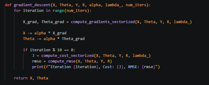
Gradient Descent

Right now, let’s recap where we are:

We have constructed a user–movie ratings matrix, initialized our model parameters randomly, and computed the cost to measure how far our predictions are from actual ratings. We then derived the gradients, which tell us how the cost changes with respect to each parameter.

Now comes the key step: updating the parameters to reduce this error.

Instead of directly modifying the cost, we adjust the parameters (movie features and user preferences). The gradient tells us the direction in which the cost increases the most, so to reduce the error, we move in the opposite direction.

This is done using gradient descent:

Parameter = Parameter − (learning rate × gradient)

The learning rate controls how big of a step we take in that direction. Over multiple iterations, these updates gradually reduce the cost and improve the model’s predictions.

Once we tune the parameters using Gradient Descent, we can use these to make predictions!

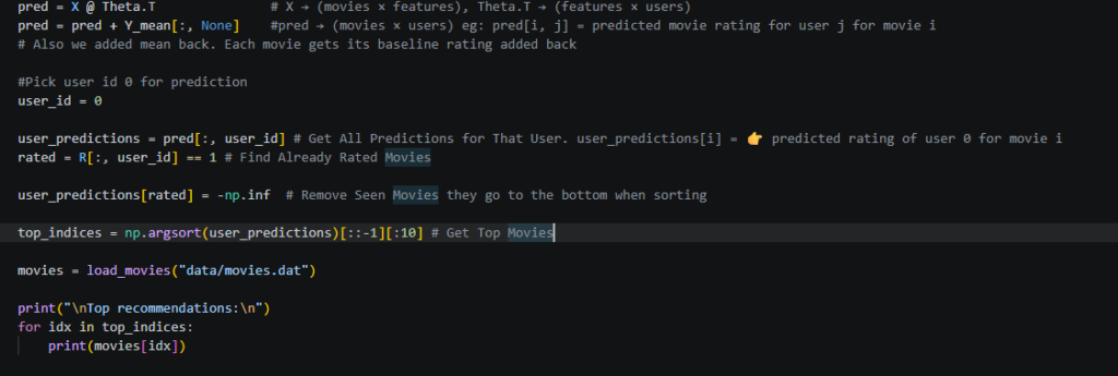
Make Predictions

Below is the screenshot that helps make prediction for a particular user. Read the comments (very helpful). I add comments to understand the flow so go through them –

X, Θ → learn patterns
↓
X @ Θᵀ → predict ratings
↓
+ mean → restore scale
↓
pick user → extract predictions
↓
remove seen → filter
↓
sort → rank
↓
map → readable movies

We mapped the names of the movies from movies data file using load_movies method.
Here are the results –

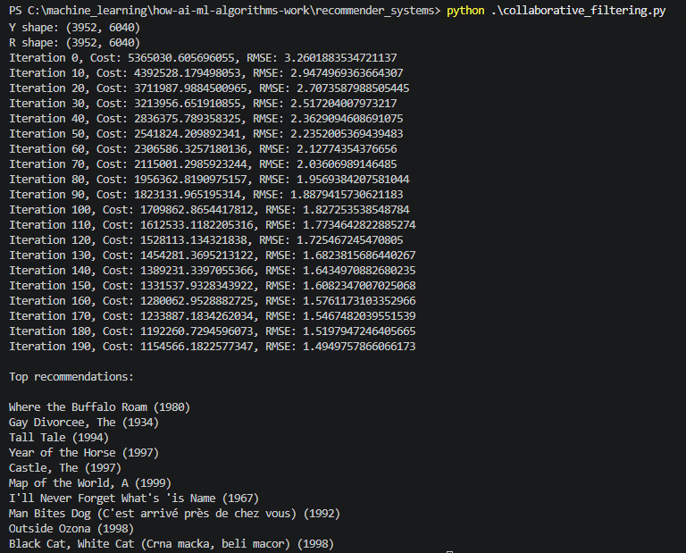
We just saw a complete recommender system working and recommending movies to users.
Isnt this great! Now what we have implemented is complete recommender system from scratch and how it is working but this is not production ready.

To make this production-ready, we would incorporate user and item bias terms, tune hyperparameters like learning rate and regularization, and evaluate performance using validation data. Additionally, handling cold-start users and scaling the system efficiently are critical for real-world deployment.

Now there are some drawbacks of Collaborative Filtering algorithm and there is another Content Based Filtering for recommender system so in next blog we will Implement that and we can explore product ready method of a recommender system in that one as well.

All symbols and functions used in the blog and code –

Variables

Symbol	Meaning
Y	Ratings matrix (movies × users)
R	Indicator matrix (1 if rating exists, else 0)
X	Movie feature matrix (movies × features)
Theta (Θ)	User preference matrix (users × features)
x(i)	Feature vector for movie i
theta(j)	Preference vector for user j

Predictions

Symbol	Meaning
Y_hat	Predicted ratings matrix
r_hat(i, j)	Predicted rating for user j on movie i
theta(j)^T x(i)	Dot product (prediction formula)

🔹 Error & Cost

Symbol	Meaning
e(i, j)	Prediction error = predicted − actual
J	Cost function (total error)
1/2 * e^2	Squared error term
lambda (λ)	Regularization parameter

Gradients

Symbol	Meaning
dJ/dx(i)	Gradient w.r.t movie features
dJ/dtheta(j)	Gradient w.r.t user preferences
e(i,j) * theta(j)	Gradient contribution for movie
e(i,j) * x(i)	Gradient contribution for user

Optimization

Symbol	Meaning
alpha (α)	Learning rate
gradient (∇J)	Direction of steepest increase

Updates

Symbol	Meaning
X = X − alpha * X_grad	Update movie features
Theta = Theta − alpha * Theta_grad	Update user preferences

Normalization

Symbol	Meaning
mu(i)	Mean rating for movie i
Y_norm	Normalized ratings
prediction + mu	Final prediction after adding mean back

Evaluation

Symbol	Meaning
RMSE	Root Mean Squared Error
sqrt(mean(e^2))	RMSE formula

Vectorization

Symbol	Meaning
X @ Theta.T	Full prediction matrix
(pred − Y) * R	Masked error matrix
error @ Theta	Gradient for X
error.T @ X	Gradient for Theta

For now, go ahead and implement a recommender system (you can chose a different dataset one that you like). I will see you next time 🙂