Introduction
A neural network in machine learning is a computational model inspired by the structure and functioning of the human brain. It consists of interconnected nodes, or “neurons,” organized into layers. It is said that it is inspired by the structure and functioning of the human brain but I believe the latter to be false as we do not even know how human brain works. It is tough to make a concrete statement on how human brain works so let us just begin with the structure and components of a neural network –
- Input Layer: This is where the model receives input data. Each neuron in this layer represents a feature or attribute of the data.
- Hidden Layers: These layers process the input data through weighted connections. Each neuron in a hidden layer applies a nonlinear activation function to the weighted sum of inputs, allowing the network to learn complex patterns.
- Output Layer: This layer produces the final prediction or classification based on the processed data. The number of neurons here corresponds to the number of possible output classes or values.
- Weights and Biases: Each connection between neurons has an associated weight, which adjusts during training to minimize the error in predictions. Biases are added to the weighted sums to help the network fit the data better.
- Activation Functions: These functions introduce non-linearity into the model, allowing it to capture complex relationships in the data. Common activation functions include ReLU (Rectified Linear Unit), Sigmoid, and Tanh.
- Training: Neural networks learn through a process called backpropagation, where the model adjusts its weights and biases based on the error between its predictions and the actual values. This is done using optimization algorithms like Gradient Descent.
Types of Neural Networks (6 Most Used)
- Feedforward Neural Networks (FNNs)
- Convolutional Neural Networks (CNNs)
- Recurrent Neural Networks (RNNs)
- Generative Adversarial Networks (GANs)
- Autoencoders
- Transformer Networks
Benefits of Deep Learning
- Feature Extraction:
- Automatic Feature Learning: Deep learning models, especially neural networks with multiple layers, can automatically learn and extract relevant features from raw data. This reduces the need for manual feature engineering.
- Automatic Feature Learning: Deep learning models, especially neural networks with multiple layers, can automatically learn and extract relevant features from raw data. This reduces the need for manual feature engineering.
- Handling Complex Data:
- High-Dimensional Data: Deep learning is effective in dealing with high-dimensional data such as images, audio, and text, where traditional methods might struggle to capture intricate patterns and relationships.
- High-Dimensional Data: Deep learning is effective in dealing with high-dimensional data such as images, audio, and text, where traditional methods might struggle to capture intricate patterns and relationships.
- Improved Accuracy:
- State-of-the-Art Performance: Deep learning models often achieve superior performance on complex tasks compared to traditional machine learning algorithms, particularly in fields like image and speech recognition.
- State-of-the-Art Performance: Deep learning models often achieve superior performance on complex tasks compared to traditional machine learning algorithms, particularly in fields like image and speech recognition.
- Scalability:
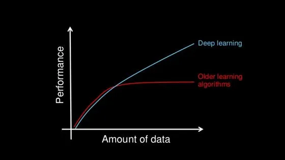
- Large Datasets: Deep learning models can leverage large amounts of data to improve their performance. As the size of the dataset increases, the model can continue to learn and adapt.
- Large Datasets: Deep learning models can leverage large amounts of data to improve their performance. As the size of the dataset increases, the model can continue to learn and adapt.
- Versatility:
- Wide Range of Applications: Deep learning is applicable to a variety of tasks, including image classification, natural language processing, object detection, generative models, and more.
- Wide Range of Applications: Deep learning is applicable to a variety of tasks, including image classification, natural language processing, object detection, generative models, and more.
- Improving Over Time:
- Continuous Improvement: With advancements in hardware (e.g., GPUs) and algorithms, deep learning models continue to improve in terms of performance, efficiency, and capabilities.
- Continuous Improvement: With advancements in hardware (e.g., GPUs) and algorithms, deep learning models continue to improve in terms of performance, efficiency, and capabilities.
The above benefits indicate that older algorithms become inefficient over time but deep learning continues to perform well.
How Neural Network Works?
At last, we arrive at the real deal. Each neuron takes input data, processes and passes it on to the other. That is it. Thank you for reading. Just Kidding, let us take a better look. As the data moves through the network, the connections between the nodes are strengthened or weakened, depending on the patterns in the data. This allows the network to learn from the data and make predictions or decisions based on what it has learned.
Look at the image below –
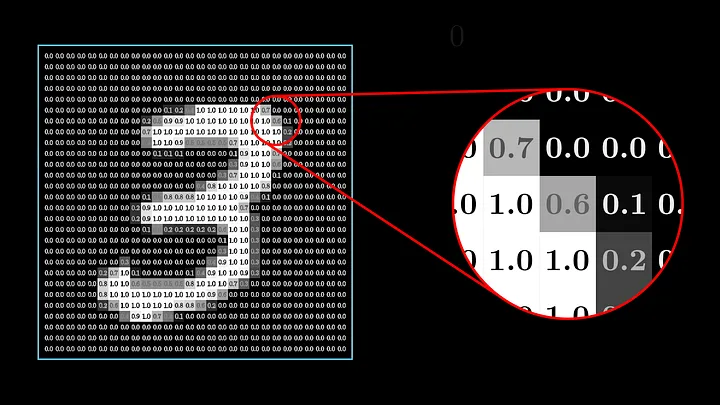
The white pixels together make up the digit 3. This is our input. This image is 28×28 in dimension. This means it has total of 784 pixels. In my notebook, the data has a shape of (42000, 785) meaning it has 42000 rows and 785 columns. 785 columns represent 784 features (pixels in a 28×28 image) and 1 label.
You can find everything in the notebooks attached.
Now if you look at the notebooks where the libraries are used and MNIST dataset is downloaded and used directly from keras data sets using tf.keras.datasets.mnist.load_data(), you will find the shape of data initially is (60000, 28, 28). We reshape this to (60000, 784). It is visualized below –

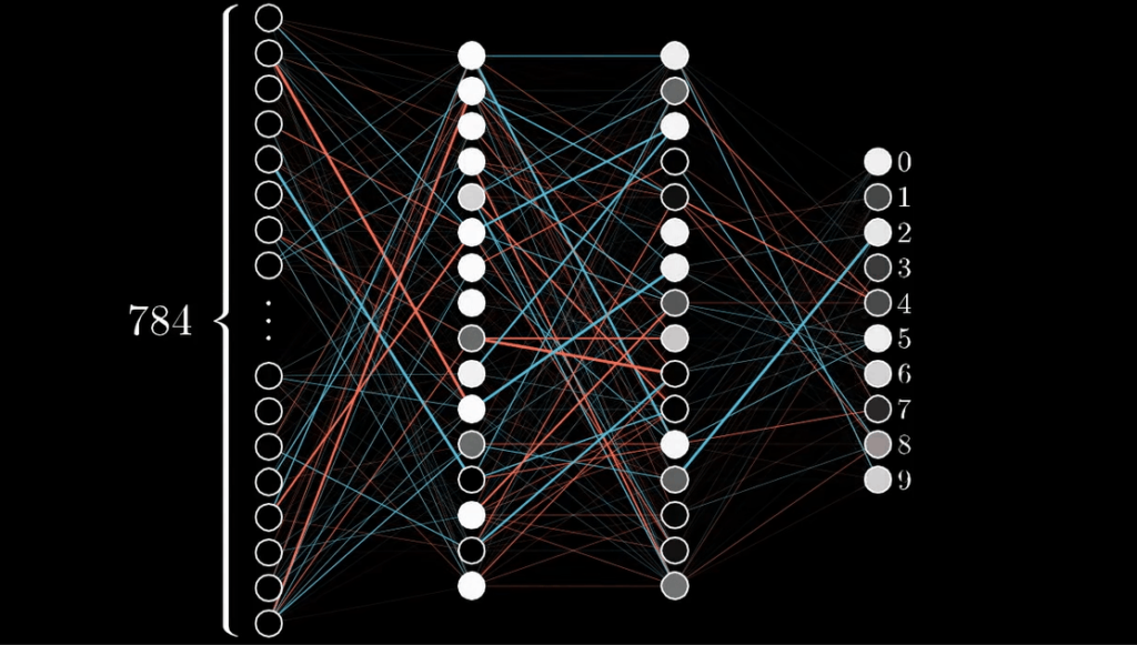
First layer is Input layer with 784 features / pixels
Now our model consist of only a single hidden layer but I could not find any animations representing that so imagine there are only three layers (Input, Hidden Layer, Output Layer).
Each pixel has a value from 0-255 depending on the brightness of the pixel.
We convert the values to 0-1 by dividing the values by 255.
Below is the image of the network and signals going through neurons for better understanding. White are near 1 and darker are near 0.
Process Step By Step
Forward Propagation
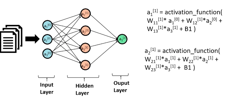
Forward propagation in a neural network involves passing input data through the network’s layers, where each layer applies weights, biases, and activation functions to compute the output. The process continues from the input layer to the output layer, producing the final prediction or result.
Refer to the notebook –
Input layer a[0]a[0] will have 784 units corresponding to the 784 pixels in each 28×28 input image. A hidden layer a[1]a[1] will have 10 units with ReLU activation, and finally our output layer a[2]a[2] will have 10 units corresponding to the ten digit classes with softmax activation.
It looks complex but it is simple. Similar to what we did in regression, wx+b. We apply this for each layer with an activation and send that data forward in the next. The hidden layer uses ReLU activation function which is also implemented in the notebook. We will go deeper in activations in later blogs. For output layer, we use softmax activation. You can imagine softmax activation as a generalization of logistic regression.
NOTE: Comments in the notebook can be very useful.
Forward propagation
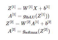
Goal: To calculate the output of the neural network by passing the input through the network layers.
- Input to Hidden Layer Calculation:
W[1]: Weights matrix for the hidden layer, shape (10, 784).X(orA[0]): Input data, shape (784, m), where 784 is the number of input features (pixels), andmis the number of examples.b[1]: Bias vector for the hidden layer, shape (10, 1).Z[1]: The weighted input to the hidden layer, shape (10, m).
- Activation of the Hidden Layer:
A[1]=gReLU(Z[1])A[1]: Activations of the hidden layer, shape (10, m), using the ReLU activation function.
- Hidden Layer to Output Layer Calculation:
Z[2]=W[2]A[1]+b[2]W[2]: Weights matrix for the output layer, shape (10, 10).A[1]: Activations from the hidden layer, shape (10, m).b[2]: Bias vector for the output layer, shape (10, 1).Z[2]: The weighted input to the output layer, shape (10, m).
- Output Layer Activation (Softmax):A[2]=gsoftmax(Z[2])
A[2]: The output of the network, shape (10, m), where each column represents the probabilities of the input belonging to each of the 10 digit classes.
Backward Propagation
Backward propagation involves computing the gradient of the loss function with respect to each weight by propagating the error backward through the network. This gradient is then used to update the weights and biases to minimize the loss.
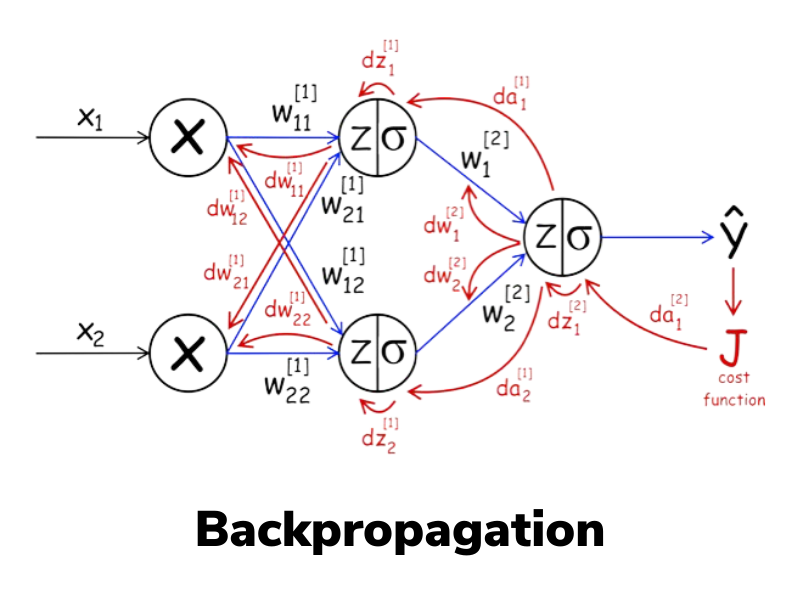
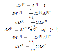
Goal: To calculate the gradients of the loss function with respect to the weights and biases, which will be used to update the parameters.
- Gradient of the Loss with Respect to
Z[2]:dZ[2]=A[2]−YdZ[2]: The error term for the output layer, shape (10, m).Y: True labels, one-hot encoded, shape (10, m).
- Gradient of the Loss with Respect to
W[2]:dW[2]=1mdZ[2]A[1]TdW[2]: Gradient with respect to the weights of the output layer, shape (10, 10).
- Gradient of the Loss with Respect to
b[2]:dB[2]=1/m∑dZ[2]dB[2]: Gradient with respect to the biases of the output layer, shape (10, 1).
- Gradient of the Loss with Respect to
Z[1]:dZ[1]=W[2]TdZ[2]⋅g′[1](Z[1])dZ[1]: The error term for the hidden layer, shape (10, m).g'[1](Z[1]): Derivative of the ReLU activation function applied toZ[1].
- Gradient of the Loss with Respect to
W[1]:dW[1]=1mdZ[1]A[0]TdW[1]: Gradient with respect to the weights of the hidden layer, shape (10, 784).
- Gradient of the Loss with Respect to
b[1]:dB[1]=1/m∑dZ[1]dB[1]: Gradient with respect to the biases of the hidden layer, shape (10, 1).
Please refer to the lines in the expression above, Writing mathematics in text is tough and should not be legal.
Parameter Updates

Just update the parameters by subtracting the derivative (don’t forget the learning rate).
NOTE: Reminder to refer notebook for better experience.
Putting It All Together (Gradient Descent)
In gradient descent, we put everything together. This function performs gradient descent to optimize the weights and biases of the network over a specified number of iterations.
- Initialize Parameters:
W1, b1, W2, b2 = init_params()initializes the weights and biases for the network.
- Iterate:
- The loop runs for the specified number of iterations.
- Forward Propagation:
Z1, A1, Z2, A2 = forward_prop(W1, b1, W2, b2, X)computes the forward pass, obtaining activations for each layer.
- Backward Propagation:
dW1, db1, dW2, db2 = backward_prop(Z1, A1, Z2, A2, W1, W2, X, Y)computes the gradients of the loss with respect to the weights and biases.
- Update Parameters:
W1, b1, W2, b2 = update_params(W1, b1, W2, b2, dW1, db1, dW2, db2, alpha)updates the weights and biases using the computed gradients and the learning ratealpha.
- Monitor Progress:
- Every 10 iterations, the function prints the current iteration number and the accuracy of the model on the training data.
Output: The optimized weights and biases (W1, b1, W2, b2) after the specified number of iterations.
Making Predictions
After training our model, it is the moment of truth. Make predictions on the data and test. You can also plot the image as I did in the notebook for visualization.
4 examples are attached in the notebook.
Neural Network Implementation from Scratch.
NOTE: Notebook containing tensorflow implementation is shared at the end.
Conclusion
Both notebooks are attached, one with neural network implementation from scratch and another using tensorflow. Same layer architecture are used in both the notebooks for better comparison.
Some terms, functions and optimizers are not explained in the blog as it will be bigger and too much at a time but the tensorflow version as you can see is more accurate and faster because of the these things. For example, ADAM optimizer over gradient descent provides better speed and accuracy as it adjust the learning rate accordingly. We will talk about these later.
To utilize this to a better extent, try creating a neural network yourself. It looks complex from outside but it is much simpler (basic neural network).
We will keep talking about machine learning.
Until Next Time ^^
Notebook (Implementation from scratch) – https://www.kaggle.com/code/innomight/digit-recognizer-from-scratch-with-explanation
Notebook (Implementation using TensorFlow) – https://www.kaggle.com/code/innomight/digit-recognizer-using-tensorflow
Previous Blogs –
Regression Model – https://vaibhavshrivastava.com/how-linear-regression-model-actually-works/
Feature Engineering – https://vaibhavshrivastava.com/the-importance-of-feature-engineering-in-machine-learning/
Logistic Regression – https://vaibhavshrivastava.com/logistic-regression-from-basics-to-code/
Scaling Algorithms – https://vaibhavshrivastava.com/scaling-features-how-scaler-works-and-choosing-the-right-scaler/

Comments