How Regression Model Actually Works

Try to fit a straight line through the points given below –

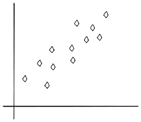
The line closest to fit the data points above would look something like this – (Suppose this is a graph between price and size of houses)

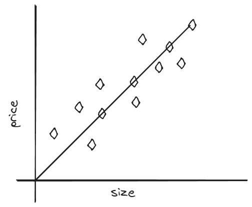
We will call the data used to train a model a training set. Single training example would be (x, y).
(x^i, yⁱ) = i^th training example.

Flow from training set to prediction –

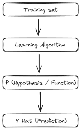
Y hat (written as ŷ) is the prediction or estimate.

How to represent the function f. What is the math formula to compute f?)
As seen above, assuming f to be a straight line, 

f_{w, b}(x) = wx + b

f_{w, b}(x) = wx + b means f is a function which takes x as input and depending on w and b, it will predict ŷ.

f(x) = wx + b

Linear regression with one variable is also called univariate linear regression.

To implement linear regression, first key step is to define something called Cost Function.
Cost Function will tell us how good model is doing.

What is a Cost Function and What Does it Do?

We saw prediction of y hat will depend on the values of w and b.
Just for simplicity sake, let us make 2 graphs with slope 0 then bias 0. w is the slope and b is the intercept.

w = 0, y = 1.5

w = 0.5, y = 0

We need to find the closest w and b for the function to go closest through the points as we saw earlier we want to draw the best possible lines that can cover the most points.

For this we construct a cost function.

Cost Function

To measure how well a choice of w and b fits the training data you have a cost function J -> measures differences between model’s prediction (y hat) and true values (y).

Cost function takes a prediction y hat and compares to target y by taking error (differense of prediction and target that is (y hat – y)

Σ (sigma) (Summation) of (all the predictions – target of the data set)² / m (no of training examples)

– Dividing by m to compute average.
– Algorithms generally divide by 2m to make later calculations look neater
– J_w,b = (Σ (sigma) (Summation) of (all the predictions (ŷ) – target of the data set (y))²) / 2m (no of training examples)

There are different cost functions for different applications and algorithms.

J_w,b = 1/2m * (f_{w, b}(x)ⁱ – y⁽ⁱ⁾)²

Goal –
Linear Regression would try to find values for w and b and make J as small as possible. Minimize J(w, b)

Visualizing Cost Function

Suppose we only have w and no b.
Cost Function Graph is of U-Shape.

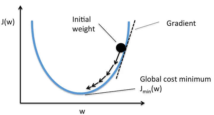
Our goal is to minimize J as we saw earlier.

If we have b along with w then we have 2 parameters and J so the graph will be of similar shape but in 3 dimensions as shown below

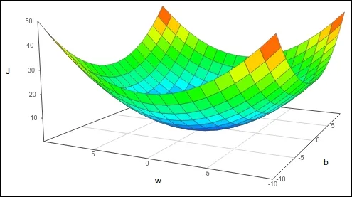
This can also be visualized in contour graph (take the above graph and cut horizontally) but we will discuss this some other time.

Gradient Descent

Our goal as seen multiple times is to minimize J. This is an algorithm that will help us do that. An algorithm to help you find min(J(w,b).

Gradient Descent can be used to minimize any function not just linear regression.

Outline –
1. Start with some w, b.
2. Keep changing w and b to reduce J(w, b) until we settle at or near minimum.

Note: J not shaped like a parabola can have more than 1 minima.

Implementing Gradient Descent

Imagine you are on top of a hill and you want the best way to climb down. You need to figure out the direction and how big of a step you can take so you do not fall down or not too slow to run out of food. Now in place of that hill, take the parabola we saw above. You want to go to that bottom of that parabola. You need derivative of J right? So we want to adjust w in such a way that we get to minimum in the best possible way.

w = w – alpha (d/dw of J(w,b))

Alpha – Learning Rate. It is a number between 0 and 1 and tell the size of change (size of step).
same with b.

b = b – alpha (d/dw of J(w,b))

We are going to use this until convergence. So, we have –

Repeat Until Convergence {
w = w – alpha (d/dw of J(w,b))
b = b – alpha (d/dw of J(w,b))
}

Note: We need to do simultaneous update so when you code it out take temporary variables so you do not change value of b with new value of w and vice versa.

Visualization helps us to understand this better so let us take a parabola again.

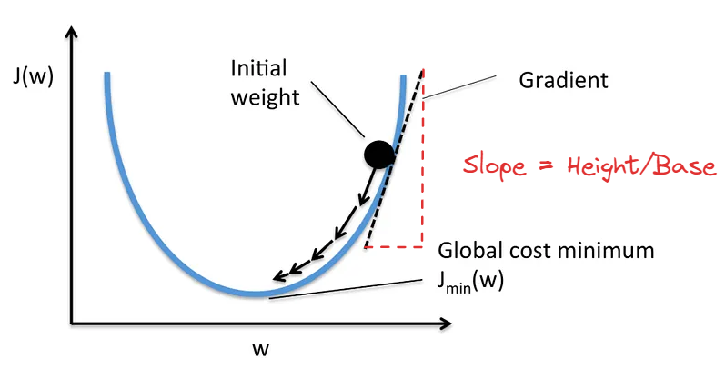
Note: From the diagrams above, you must have understood that positive slope will mean
w = w – alpha * (Positive Number), and negative slope will mean
w = w – alpha * (Negative Number)

Above note can help you visualize where you are on the parabola, left or right of the minima.

Choice of Learning Rate alpha will impact efficiency. If it is too small, Gradient descent will be slow.
If it is too large, Gradient descent may overshort and never reach minima.

Now after finding out the best w and b you can run your prediction analysis.

If you have any questions, you can comment below or message me directly over any platform.
Until next time ^^