Logistic Regression: From Basics to Code

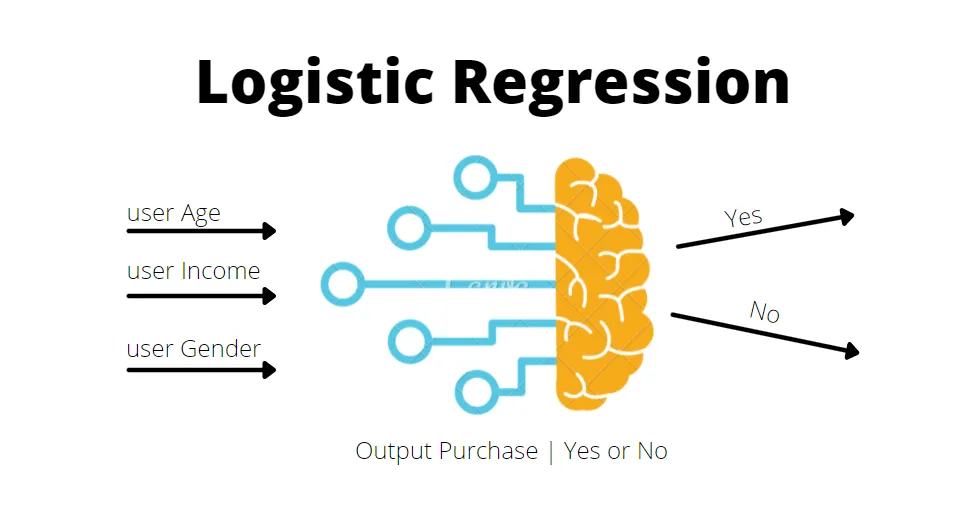
Is it a dog or a cat? Is it male or a female? (Just kidding)
Logistic Regression can help you in tasks like above. Tasks that involve classification. In my recent blog, I have discussed about how regression works. We will apply same principles here too but with little tweaks and adjustments. We will implement Logistic Regression from scratch which will be insightful in looking into how Logistic Regression actually works (No Scikit-Learn or Tensorflow).

What are we implementing?

I picked up a dataset from Kaggle which has information about people, their area income, their time spent of site etc. and if they clicked on the Advertisement or not. So it is a dataset we will use to train our model to predict if a person will click on the ad or not. We will implement Logistic regression from scratch. That will include the following –

• Loading the dataset
• Splitting the dataset
• Standardization of data
• Exploring data
• Visualizing some aspects of data
• Visualizing Sigmoid Function
• Implementing methods for finding Sigmoid, Loss, Gradients
• Finally Gradient Descent and Prediction

Logistic Regression Basics

Logistic Regression is a supervised algorithm used to predict the probability of the dependent variable or put the result in a class. Example: Cat or Dog (2 classes)

Types of Logistic Regressions –

Binary Logistic Regression:
The dependent variable has only 2 possible outcomes/classes.
Example-Male or Female.

Multinomial Logistic Regression:
The dependent variable has 3 or more possible outcomes/classes without ordering.
Example: Predicting food quality.(Good, Great and Bad).

Ordinal Logistic Regression:
The dependent variable has 3 or more possible outcomes/classes with ordering. Example: Star rating from 1 to 5

Logistic Regression Usage

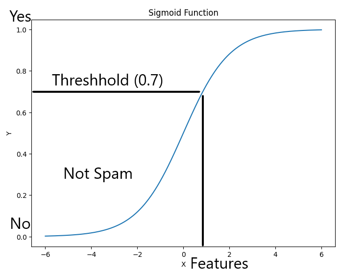
It is the single most widely used Classification Algorithm. We try to fit values in an S shaped curve (We will learn about this in a bit) that creates a threshold and values in the respective thresholds are classified in classes. For example Is the Email Spam/Fraud? (See below graph)

In the above graph, we set a threshold of 0.7. Values above this are considered Spam Email and below Not Spam. This is how we classify anything using logistic regression. You see above the graph says Sigmoid Function. Let us see what Sigmoid Function is.

Sigmoid Function

Sigmoid function has many use cases but for now let us focus on the main use which is – It maps any real-valued number into a value between 0 and 1. The sigmoid function is defined by the formula:σ(x)=

Value of e is 2.71. It keeps on going after .71 like pi. It is an irrational number used mostly in logarithm concepts.

Key Characteristics:

1. S-Shaped Curve: The sigmoid function produces an “S”-shaped curve when plotted, smoothly transitioning from 0 to 1 as the input value moves from negative to positive infinity.
2. Output Range: The function outputs values strictly between 0 and 1. For very large negative inputs, the output is close to 0, and for very large positive inputs, the output is close to 1.
3. Smooth Gradient: The derivative of the sigmoid function is smooth and non-zero, which helps in gradient-based optimization methods like gradient descent.

Why Squared Error Loss Function Does not Work With Logistic Regression –

We saw squared error cost function in this blog but it is not ideal for Logistic Regression because –
f^w,b (x) = 1 / (1 + (e^{-(w.x + b)} )
In squared error cost function –
J^w,b = 1/2m * (fw, b(x)i – y(i))²
where f^w,b (x) = w.x + b
so the graph between J and w comes out like –

If we use same Cost function with logistic regression with f^w,b (x) = 1 / (1 + (e^{-(w.x + b)} ), the graph would be non convex and we will have too many local minimas.

Logistic Loss Function

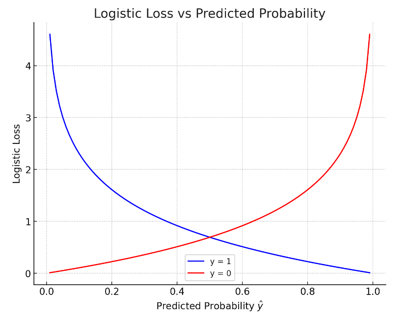
The logistic loss function is derived from the principle of maximum likelihood estimation (MLE) in a probabilistic framework. It intuitively penalizes the model more as the predicted probability deviates further from the actual label, thereby guiding the model to make better predictions during training.

Logistic regression model – predicts y_hat using the sigmoid function we saw above

Intuitively, if y (target variable) is 1, we want y_hat (predicted value) to be close to 1.
Logistic loss function L(f_w,b(xⁱ, yⁱ ) =
if yⁱ = 1,
L(f_w,b(xⁱ, yⁱ ) = -log f_w,b(xⁱ )
if yⁱ = 0,
L(f_w,b(xⁱ, yⁱ ) = -log (1 – f_w,b(xⁱ ) )

It measures how well you are doing on entire training set. So the graph will look like this –

There can be a separate blog talking about losses and different loss functions so let us just wind up the logistic loss function and give the simplified loss function.

Simplified Loss Function –
L(fw,b(xi, yi ) = -yⁱ . log(f(xⁱ)) – (1 – yⁱ) . log(1 – f(xⁱ))
if y = 1,
L(fw,b(xi, yi ) = -1 . log(f(xi)) – (1 – 1) . log(1 – f(xi)) = – log(f(xⁱ))
if y = 0,
L(fw,b(xi, yi ) = -0 . log(f(xi)) – (1 – 0) . log(1 – f(xi)) = – log(1 – f(xⁱ))

Final Cost Function –
J(w, b) = 1/m ∑ (L(f(xi, yi ))

Gradient Descent

Gradient Descent looks similar for both linear regression and logistic regression.
Refer the gradient descent part of my recent blog How Regression Model Works for detailed info.
The change would be –
In linear regression, f(x) = w.x + b
In logistic regression, f(x) = 1 / (1 + (e^{-(w.x + b)} )

Logistic Regression Implementation (Click on Advertisement Prediction)

Dataset from kaggle.
Complete implementation can be found in the below Kaggle Notebook.
https://www.kaggle.com/code/innomight/logisticregression?kernelSessionId=191861553

Conclusion

Logistic regression is a fundamental method for binary classification, transforming linear combinations of features into probability estimates. Its simplicity and interpretability make it a go-to model for many applications. By minimizing the logistic loss, it ensures predictions align closely with actual outcomes, providing both predictive power and insights into data.

I hope this blog gave you some valuable insights.
Until next time ^^